This is the second of two articles on BlueDot Technical AI Safety Puzzle #1. For the first two questions, see The Country Basin.
Takeaway
Probably yes.
With three reserved channels and explicit geometric and causal constraints, a small MLP can encode country on a prescribed sphere shell or helix tube while preserving task performance and being causally used.
- Reserved code
- 3 channels
- Country AUC
- 0.9994 / 0.9936
- Causal delta
- 3.42 / 2.14
About BlueDot’s Puzzle #1
BlueDot’s Technical AI Safety Puzzle #1 provides a trained five-layer MLP that performs multi-label classification over eight binary features using mean-pooled representations from a sentence transformer. The puzzle indicates nonlinear behaviour at the output of the third ReLU, denoted as $\ell$, and asks participants to:
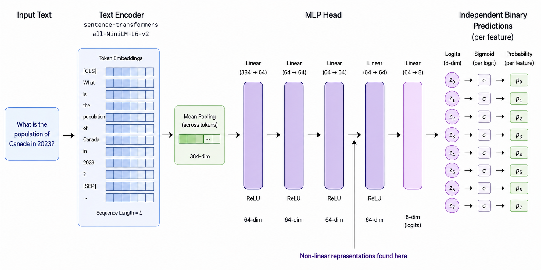
- Find the nonlinear feature, denoted as $f$.
- Explain the geometry used by the model at $\ell$ to represent $f$.
- Train a new model with a more interpretable representation.
This article addresses the third task. I train a new small MLP and constrain country to use a chosen three-dimensional manifold while testing whether the classifier actually relies on that code.
Can We Choose the Manifold Before Training?
For question 3, I want to make the representation interesting in a controlled way.
Can we choose a representation geometry first, then train the model so that the feature follows that geometry while still solving the original task?
This is inspired by recent work showing that neural representations can contain meaningful curved geometries, not only linear directions. Gurnee et al. [1] study counting manifolds in language models, where internal computation manipulates structured manifolds. Wurgaft et al. [2] study manifold steering, where steering along a learned curved representation can be more faithful than steering along a straight line. I use the same broad intuition, but in the opposite direction: instead of discovering a manifold after training, I build a small manifold code first and ask the model to use it.
The important difference is that I do not want the manifold to be decorative. The target feature should actually be decoded from that geometry. So the experiment needs to test not only:
Did the hidden activations form the desired shape?
but also
Did the model actually use that shape to solve the task?
In this article, I show how I gradually achieved this. I train a new five-layer MLP with ReLUs. The target feature, country, is encoded through a reserved 3D geometry code at hidden layer 2. I guide the model to use either a sphere shell or helix tube representation within a controlled 3D subspace while preserving task performance and passing causal-use checks.
The word “use” is the key. A manifold can be visible and still be useless. A model could place points in a desired subspace while solving the task from a hidden linear shortcut somewhere else. So here is my design:
- The geometry is specified before training.
- The learned geometry code matches the specified geometry.
- The original eight-label task still works.
- Easy shortcuts, especially linear access and complement-only access, are weak.
- Intervening on the geometry code changes the country prediction.
The rest of this article describes the stage-by-stage process used to establish these checks.
Notation
Notation used throughout this article.
| Symbol | Meaning |
|---|---|
| Data and labels | |
| $i,j,k, K, m$ | Example, anchor, or path-step index; $K$ is the number of path points and $m$ is the number of positive-negative pairs. |
| $x_i, e_i$ | Input text and its mean-pooled sentence-transformer embedding. |
| $f, f^\star$ | A puzzle feature and the target feature, with $f^\star=\text{country}$. |
| $y_i^f, y_i, \mathbf y$ | Binary label for feature $f$ on example $i$; $y_i=y_i^{f^\star}$ when unambiguous, and $\mathbf y$ is that target-label vector across a batch. |
| $\hat y_i^f$ | Model prediction for feature $f$ on example $i$. |
| $P, N, (p_j,n_j)$ | Held-out positive and negative index sets, and their paired indices for swap interventions. |
| Target manifolds and distributions | |
| $\mathcal{G}$ | Chosen geometry family: a sphere shell or helix tube. |
| $Q_1, Q_0, Q_{\mathrm{mix}}$ | Positive, negative, and class-mixture target geometry distributions. |
| $B, n, N, M$ | Minibatch, its number of points, the number of examples in the relevant loss batch, and the number of eligible label groups in ClassOT. |
| $Z_1, Z_0, Z_y, Z_B$ | Learned geometry-code sets for each class or for minibatch $B$. |
| $A_y, \alpha_j^y, \alpha_i^y$ | Anchor set and a sampled target point for class $y\in\{0,1\}$; its index follows the associated anchor or example. |
| $u, \rho, r_1, r_0, \delta_\rho$ | Sphere direction, sampled radius, positive/negative target radii, and radius-noise width. |
| $t, T, \beta, \varphi$ | Helix position, maximum helix position, vertical pitch, and tube cross-section angle. |
| $c(t), n_1(t), n_2(t)$ | Helix centerline and its two local cross-section directions. |
| $g(\eta), \eta, \xi_i, \mathbb{S}^2$ | Raw geometry map, its sampling parameters, a hypothetical pointwise coordinate, and the unit sphere. |
| $\sigma_{\mathcal G}, \sigma_{\mathrm{sphere}}, \sigma_{\mathrm{helix}}$ | Geometry-normalization scales for the chosen family, sphere shell, and helix tube. |
| $\operatorname{Unif}[a,b], \pi$ | Uniform distribution over $[a,b]$ and the country-positive rate. |
| Model and representation | |
| $\ell, h_i^2$ | Investigated layer in the original puzzle and the new model’s post-ReLU hidden-layer-2 state. |
| $a_i, a_\theta(e_i), \theta$ | Reserved preactivations, learned coordinate head, and its trainable model parameters. |
| $u_i, v_i, \theta_i, \rho_i, R_{\max}$ | Learned sphere direction components or learned helix coordinates, plus the maximum permitted radius. |
| $z_i, r_i, \bar r$ | Three-channel geometry code, 61-channel complement, and minibatch mean complement. |
| $\bar h_j^2,\ \bar y$ | Batch means of hidden2 channel $j$ and the target label, used in correlation penalties. |
| $G_{\mathcal{G}}, b_{\mathcal{G}}$ | Fixed bottleneck map for $\mathcal{G}$ and its positive post-ReLU offset. |
| $h_i^+,h_i^-,\ \tilde h_i^2$ | Positive- and negative-anchor edited states, and a generic intervened hidden state. |
| $h_i^{\mathrm{ctx}}, h_i^{\mathrm{neu}}$ | Tail-fitting context and neutral states with a frozen example-specific or mean complement. |
| $z^{(k)},\ h^{(k)}$ | Geometry code and hidden state at path step $k$ during a deterministic intervention. |
| $C(\cdot), C_{f^\star}(\cdot)$ | Model tail from hidden2 to logits and its country-logit component. |
| Objectives and diagnostics | |
| $\mathcal{L}_{\mathrm{task}}$ | Original eight-label binary cross-entropy task loss. |
| $\operatorname{OT}_{\varepsilon}, \Pi, C_{ij}, \mathbf 1, \varepsilon$ | Entropic optimal-transport objective, transport plan, pairwise transport cost, all-ones vector, and entropy weight. |
| $d_0(z), d_1(z), s_{\mathrm{geo}}(z), k, \gamma$ | Squared distances to the negative and positive target radii, the logit-like geometry score and its scale factor, and the probe-score scale. |
| $\lambda_{\bullet}, \mathcal{L}_{\bullet}$ | Loss weights and the corresponding MixOT, ClassOT, radius, geometry-score, causal, tail, adversarial, and leakage losses. |
| $\operatorname{stopgrad}, \operatorname{GRL}$ | Gradient-stopping operator and gradient-reversal layer. |
| $\operatorname{BCEWithLogits},\ \operatorname{SmoothL1},\ \operatorname{Corr}$ | Binary cross-entropy on logits, the robust regression loss, and the batchwise correlation operator. |
| $a_\phi, c_\psi, \phi, \psi$ | Full-hidden and complement adversary logits, with their trainable parameters. |
| $\sigma, w, b$ | Sigmoid function and the weight and bias of the one-layer full-hidden adversary. |
| $\Delta_{\mathrm{target}}, \Delta_{\mathrm{swap}}, \Delta_{\mathrm{path}}$ | Replacement, swap, and path causal target shifts. |
| $\ell_k, M_{\mathrm{path}}$ | Country logit at path step $k$ and the fraction of path steps moving in the expected direction. |
| AUC, MAE, coverage entropy, causal target delta, specificity | Metrics for task performance, radius error, manifold coverage, causal responsiveness, and target selectivity. |
1. Define the Target Manifold Before Training
The first stage has no model. I only define what the model will later be asked to learn.
1.1 The Distributional Problem
For each example $i$, the dataset gives the binary target label $y_i^{f}$. It tells me whether country is present, but not where that example should sit on a desired manifold. For a helix, $y_i^{f}=1$ does not provide a position $t_i$, radius $\rho_i$, or tube angle $\varphi_i$. These values are not observed. This is important because if I have its coordinates $\xi_i=(t_i,\rho_i,\varphi_i)$, then I could train the model with pointwise supervision $z_i \approx g(\xi_i)$.
Instead, I use a distributional target: $Q_1$ for positive examples and $Q_0$ for negative examples. The target is:
\[\begin{aligned} Z_1 &= \{z_i : y_i^{f^\star}=1\} \quad\text{should look like}\quad Q_1,\\ Z_0 &= \{z_i : y_i^{f^\star}=0\} \quad\text{should look like}\quad Q_0. \end{aligned}\]Here, $Z_1$ and $Z_0$ are the learned geometry codes for positive and negative target examples. The model is free to choose individual placements; what matters is that the aggregate positive distribution matches $Q_1$ and the aggregate negative distribution matches $Q_0$.
This is close in spirit to Wasserstein Auto-Encoders: the encoded aggregate distribution is matched to a chosen prior instead of assigning every example a hand-written latent coordinate [3].
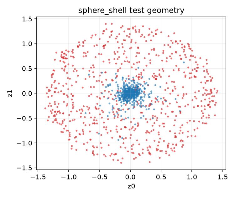
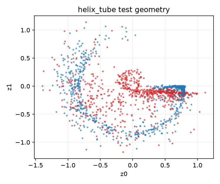
I choose two target geometries: a sphere shell and a helix tube, shown in Figure 1. Both use the same class coding: positives occupy an inner radius and negatives an outer radius while both classes span the same scaffold. This makes the label a distance-to-structure decision rather than a global direction; if positives occupied only the north pole and negatives only the south pole of one sphere, the representation would be essentially linear.
1.2 Sphere Shell
The first geometry is a sphere shell. Let $u$ be a direction sampled uniformly from the unit sphere $\mathbb{S}^2=\lbrace x\in\mathbb{R}^3:\lVert x\rVert_2=1\rbrace$, the set of points in 3-dimensional space with Euclidean norm 1.
Let $\rho$ be a radius. The raw sphere point is:
\[g_{\text{sphere}}(u,\rho)=\rho u, \qquad u\in\mathbb{S}^2\subset\mathbb{R}^3\]The positive class uses a smaller radius than the negative class:
\[Q_1:\rho\approx r_1, \quad Q_0:\rho\approx r_0, \quad r_1<r_0.\]Here, $r_1$ is the target radius for positive examples and $r_0$ is the target radius for negative examples. $\approx$ means the sampled radius is concentrated near that value, not exactly fixed at that value. In this experiment, I use
\[r_1=0.30,\quad r_0=0.85.\]The sphere therefore encodes country by inner versus outer shell, not by direction (see Figure 1).
1.3 Helix Tube
The second geometry is a helix tube. Let $t\in[0,T]$ be the position along the helix with a maximum value of $T$. Let $\beta$ be the vertical pitch parameter that controls how fast the helix rises (i.e. how stretched it is). The helix core curve is:
\[c(t)= \begin{bmatrix} \cos t\\ \sin t\\ \beta(t-T/2) \end{bmatrix}.\]Here, $c(t)$ is the 3-dimensional centerline of the helix.
To make a tube around the centerline, I need two directions perpendicular to the centerline. The first tube direction is:
\[n_1(t)= \begin{bmatrix} \cos t\\ \sin t\\ 0 \end{bmatrix}.\]The second tube direction is:
\[n_2(t)= \frac{1}{\sqrt{1+\beta^2}} \begin{bmatrix} -\beta\sin t\\ \beta\cos t\\ -1 \end{bmatrix}.\]The vectors $n_1(t)$ and $n_2(t)$ are the local cross-section directions around the helix. Let $\varphi$ be the angle around that tube cross-section, with $\varphi\in[0,2\pi]$. Let $\rho$ again be the tube radius. A point in the helix tube is:
\[g_{\text{helix}}(t,\rho,\varphi)=c(t)+\rho\left(\cos\varphi\,n_1(t)+\sin\varphi\,n_2(t)\right).\]The class-conditional distributions are:
\[Q_1:t\sim \operatorname{Unif}[0,T],\quad \varphi\sim \operatorname{Unif}[0,2\pi], \quad \rho\approx r_1,\] \[Q_0:t\sim \operatorname{Unif}[0,T],\quad \varphi\sim \operatorname{Unif}[0,2\pi], \quad \rho\approx r_0, \quad r_1<r_0.\]In this experiment, I use:
\[\beta=0.12,\quad r_1=0.15,\quad r_0=1.00.\]Both classes trace the same curved scaffold; country is decoded by distance to the inner or outer tube rather than by one plane (see Figure 1). I tried three turns but they were not reliably readable by the tail layer under the remaining constraints, while one turn remained learnable, usable, and testable.
1.4 Sampled Distribution
Figure 1 shows the target distributions before the model sees any examples.
Figure 1 · Chosen manifold sampler
The target distributions are specified before the model sees an example.
Loading target manifolds…
1.5 Normalization
Because the sphere and helix have different natural scales, I normalize sampled points so the experiment tests shape rather than raw norm. Let $g(\eta)$ be a raw geometry point, with $\eta=(u,\rho)$ for the sphere and $\eta=(t,\rho,\varphi)$ for the helix. With balanced classes, I define the geometry scale:
\[\sigma_{\mathcal{G}}=\sqrt{\mathbb{E}\left[\lVert g(\eta)\rVert_2^2\right]}.\]Each geometry code is then normalized:
\[z=\frac{g(\eta)}{\sigma_{\mathcal{G}}}.\]For the sphere shell:
\[\sigma_{\text{sphere}} = \sqrt{ \frac{1}{2}(r_1^2+r_0^2) + \frac{\delta_\rho^2}{12} }.\]For the helix tube:
\[\sigma_{\text{helix}} = \sqrt{ 1+ \frac{\beta^2T^2}{12} + \frac{1}{2}(r_1^2+r_0^2) + \frac{\delta_\rho^2}{12} }.\]Here, $\delta_\rho$ is the radius-noise width. Its $\delta_\rho^2/12$ contribution follows the uniform-interval variance rule $w^2/12$ [4]. The helix additionally contributes $1$ from its circular core $(\cos t,\sin t)$ and $\beta^2T^2/12$ from its centered vertical coordinate.
Before training, I draw target anchors from the normalized distributions: $\alpha_j^1\sim Q_1$ for positives and $\alpha_j^0\sim Q_0$ for negatives.
\[\alpha_j^1\sim Q_1,\quad \alpha_j^0\sim Q_0.\]2. Train the Model
2.1 Base Classifier
In this stage, I set up a base five-layer MLP classifier with ReLUs. Each text input $x_i$ is encoded by sentence-transformers/all-MiniLM-L6-v2 before mean-pooling into $e_i\in \mathbb{R}^{384}$. I then feed this representation into a five-layer ReLU MLP to get eight logit outputs. This model is trained using BCE loss
\[\mathcal{L}_{\text{task}}=-\frac{1}{N}\sum_{i=1}^{N}\sum_{f=1}^{8}\left[y_i^f\log\hat y_i^f+(1-y_i^f)\log(1-\hat y_i^f)\right].\]Here is its performance on the eight labels:
- Mean AUC: 0.9884
- Mean accuracy: 0.9616
- Country AUC: 0.9994
The target of this stage is to have an ordinary classifier that works, so later failures should come from manifold constraints rather than architecture or data handling.
2.2 Add the Geometry Bottleneck and Activation-Sign
2.2.1 Geometry Bottleneck
I reserve three hidden2 preactivations $a_i=(a_{i1},a_{i2},a_{i3})$ for a geometry code $z_i$, leaving the remaining 61 coordinates as the complement $r_i$. Three channels are the minimal space that can store a point on either target 3D manifold; more channels would make the construction less minimal, while fewer could not contain the requested geometry.
Because hidden2 is post-ReLU, its coordinates are nonnegative. I therefore add a positive offset $b_{\mathcal{G}}$ so the signed manifold code can live in this activation space:
\[h_i^2=[z_i+b_{\mathcal{G}},r_i].\]Figure 2 · The three-channel bottleneck
Three channels receive a chosen manifold; the remaining 61 channels are the complement to guard against.
Choose a component to inspect the role it plays in the design.
Let $\mathcal{G}$ be the chosen geometry family, either the sphere shell or the helix tube. The learned coordinate head $a_\theta(e_i)$ predicts three unconstrained values from the sentence embedding, and the fixed map $G_{\mathcal{G}}$ converts them into a valid normalized point on the selected manifold:
\[z_i=G_{\mathcal{G}}(a_\theta(e_i)).\]For the sphere bottleneck,
\[z_i=\frac{\rho_i u_i}{\sigma_{\text{sphere}}}, \quad u_i= \begin{bmatrix} \sqrt{1-v_i^2}\cos\theta_i\\ \sqrt{1-v_i^2}\sin\theta_i\\ v_i \end{bmatrix}.\]where $\theta_i=a_{i1}$ is the azimuth angle, $v_i=\tanh(a_{i2})$ is the vertical coordinate, and $\rho_i=10^{-3}+R_{\max}\operatorname{sigmoid}(a_{i3})$ has maximum allowed radius $R_{\max}$.
For the helix bottleneck,
\[z_i=\frac{g_{\text{helix}}(t_i,\rho_i,\varphi_i)}{\sigma_{\text{helix}}}\]where $t_i=T\operatorname{sigmoid}(a_{i1})$, $\varphi_i=2\pi\operatorname{sigmoid}(a_{i2})$, and $\rho_i=10^{-3}+R_{\max}\operatorname{sigmoid}(a_{i3})$.
2.2.2 Experiment
At this stage, I optimize only the original task loss:
\[\mathcal{L}=\mathcal{L}_{\text{task}}.\]The purpose is not yet to force good class geometry. I ask only:
Can the classifier survive this architectural constraint?
To test whether the reserved code contains the predefined geometry while the model still solves the task, I define four analyses alongside mean AUC and country AUC.
-
Geometry probe. It asks: if I look only at the 3D geometry point, ignoring the classifier and complement channels, can I tell whether the example is country by checking whether it sits near the positive or negative part of the target geometry? It is a fixed geometry-based readout from only the first three hidden2 channels, $z$. It:
- takes the learned 3D geometry code $z$;
- converts it back to raw geometry scale;
- measures its geometry radius:
- For sphere shell: distance from the origin;
- For helix tube: distance to the nearest point on the helix core;
- asks: is this radius closer to the positive radius or negative radius?
- computes ROC AUC between this score and country labels.
Therefore, this metric does not prove the model uses the geometry. It only proves the reserved channels contain the label in the intended geometric way.
-
Coverage entropy. It asks: do the learned geometry points spread across the intended shape, or do they collapse into one small patch?
- For sphere shell, it
- takes the learned 3D geometry points
- computes their azimuth angle in the x-y plane
- puts those angles into 8 bins around the circle
- computes normalized entropy of the bin counts
→ High coverage entropy means the points wrap around the shell instead of all sitting on one side.
- For helix tube, it
- finds the nearest point on the helix core for each learned geometry point
- converts that nearest point into a helix position $t$
- bins $t$ into 24 bins across the full helix
- computes normalized entropy
→ High coverage entropy means the learned points spread along the helix instead of using one small segment.
- For sphere shell, it
-
Causal target delta. It asks: if I edit only the 3 geometry channels, does the model’s own country logit move? It does this by:
- Replacing channels with positive-geometry anchors
- Replacing channels with negative-geometry anchors
- Running the tail on both edited hidden states
- Computing their mean differences
A large positive value means the model’s tail is actually listening to the geometry channels for country, while a small near-zero value means the geometry may look correct, but the tail is ignoring it.
-
Linear probe AUC. I train a linear probe on the country’s activations and get its AUC.
2.2.3 Results
Table 1. Model behaviour after adding the geometry bottleneck. Higher is better unless marked ↓.
| Geometry | Mean task AUC (↑) |
Country AUC (↑) |
Geometry probe AUC (↑) |
Linear probe AUC (↓) |
Coverage entropy (↑) |
Causal delta (↑) |
|---|---|---|---|---|---|---|
| Sphere shell | 0.9975 | 0.9995 | 0.2021 | 0.9996 | 0.7971 | 0.0187 |
| Helix tube | 0.9963 | 0.9997 | 0.1182 | 0.9997 | 0.6561 | 0.0357 |
As shown in Table 1, the model survives the bottleneck. However, causal delta scores for both geometries indicate that the model does not use the intended geometry. Instead, the model appears to route the label through other complement channels, suggesting that bottleneck alone is not enough.
On the other hand, low geometry probe AUC and low coverage entropy indicate that the geometry of country does not follow what we defined.
2.3 Add Unconditional Optimal Transport Coverage
This stage asks:
Can the learned geometry codes cover the target geometry instead of collapsing to a small region?
The bottleneck constrains each learned code to the allowed geometry family, but it does not ensure that a minibatch uses the whole geometry. In the helix setting, for example, every example can map to a valid point on the tube while almost all examples still occupy the same segment. The representation is technically on the helix, but it is not yet a meaningful representation of the feature.
To prevent this collapse, I add an unconditional mixture optimal transport (MixOT) loss. It spreads the unlabelled minibatch across the overall target geometry, without yet requiring positive examples to occupy $Q_1$ and negative examples to occupy $Q_0$. The target distribution is
\[Q_{\mathrm{mix}}=\pi Q_1+(1-\pi)Q_0,\]where $\pi$ is the positive rate of country in the training set.
For a minibatch $B$, let $Z_B=\lbrace z_i:i\in B \rbrace$ be its $n$ learned 3D geometry codes. I sample the same number of target anchors (see Section 1.4) from $Q_{\mathrm{mix}}$:
\[A_{\text{mix}}=\{\alpha_1,\ldots,\alpha_n\},\quad \alpha_j\sim Q_{\text{mix}}\]These anchors form a fresh minibatch target point cloud: both inner and outer shells for the sphere shell, and both tubes for the helix tube.
Think of learned codes as students and target anchors as seats spread across the shape. OT matches each student to a seat while requiring every seat to receive a match. If the codes crowd into one corner, many distant seats make the matching costly; if they spread across the geometry, the matching is cheaper.
Therefore, for a learned code $z_i$ and a target anchor $\alpha_j$, the transport cost is
\[C_{ij}=\lVert z_i-\alpha_j\rVert_2^2\]Entropic OT solves
\[\operatorname{OT}_{\varepsilon}(Z_B,A_{\text{mix}})=\min_{\Pi}\sum_{i,j}\Pi_{ij}C_{ij}+\varepsilon\sum_{i,j}\Pi_{ij}(\log\Pi_{ij}-1)\]subject to the balanced constraints
\[\Pi\mathbf{1}=\frac{1}{n}\mathbf{1}, \quad \Pi^\top\mathbf{1}=\frac{1}{n}\mathbf{1}.\]Here $\Pi$ is the transport plan. The first constraint assigns every learned point, and the second ensures every target anchor receives mass. This second constraint makes collapse expensive: the model cannot ignore most anchors and only match the easy ones. The entropy weight $\varepsilon$ smooths the matching for efficient Sinkhorn optimization [5].
To test whether class-conditional geometry works on its own, I replace the previous MixOT term with:
\[\mathcal{L}=\mathcal{L}_{\text{task}}+\lambda_{\text{mix}}\operatorname{OT}_{\varepsilon}(Z_B,A_{\text{mix}}).\]2.3.1 Results
In this section, I add Radius MAE to measure the mean absolute error between the learned geometry radius and the desired class radius (lower is better).
Table 2. Model behaviour after adding unconditional mixture optimal transport.
| Geometry | Stage | Mean task AUC (↑) |
Country AUC (↑) |
Geometry probe AUC (↑) |
Linear probe AUC (↓) |
Coverage entropy (↑) |
Causal delta (↑) |
Radius MAE (↓) |
|---|---|---|---|---|---|---|---|---|
| Sphere shell | Bottleneck | 0.9975 | 0.9995 | 0.2021 | 0.9996 | 0.7971 | 0.0187 | 0.7243 |
| MixOT | 0.9974 | 0.9990 | 0.5585 | 0.9993 | 0.9991 | 0.0206 | 0.3012 | |
| Helix tube | Bottleneck | 0.9963 | 0.9997 | 0.1182 | 0.9997 | 0.6561 | 0.0357 | 0.6653 |
| MixOT | 0.9975 | 0.9993 | 0.3095 | 0.9994 | 0.9942 | 0.0368 | 0.5582 |
Coverage entropy is almost perfect for both geometries, showing that MixOT prevents the codes from collapsing into a small region. However, geometry probe AUC remains weak, radius MAE remains large, and causal target delta is nearly zero.
This is expected: MixOT spreads the unlabelled batch, but does not yet tell positives to use $Q_1$ or negatives to use $Q_0$. The next stage adds that class-conditional structure.
2.4 Add Class-Conditional Geometry
This stage addresses the previous stage’s limitation:
Put positive examples in the positive part of the shape, and put negative examples in the negative part.
MixOT spreads the whole batch across the shape, but it does not assign each class to its own part. I therefore replace the shared seating chart with class-conditional matching: positives receive anchors from $Q_1$ and negatives receive anchors from $Q_0$. I also add a radius loss and a geometry-score loss to give each individual code a local training signal.
2.4.1 Class-Conditional OT (ClassOT)
For label $y\in\lbrace0,1\rbrace$, let $Z_y=\lbracez_i:y_i=y\rbrace$ be the matching learned codes in minibatch $B$, and let $A_y$ be anchors sampled from $Q_y$. The class-conditional OT is:
\[\mathcal{L}_{\text{class-OT}}=\frac{1}{M}\sum_{y\in\{0,1\}: |Z_y|\ge 2}\operatorname{OT}_{\varepsilon}(Z_y,A_y).\]Here, $M$ is the number of included label groups; a class term is skipped when fewer than two examples of that class appear in the batch.
2.4.2 Radius Loss
ClassOT gives the right distributional shape, but it can still be weak as a per-example training signal. The fixed MLP tail after hidden2 must decode country from each geometry code; a batch-level match does not necessarily give it a simple local cue for an individual example. Radius loss supplies that cue: each example should reach its class radius, not merely belong to a batch that can be matched to the right anchors.
Let $\operatorname{rad}_{\mathcal{G}}(z)$ be the geometry-specific radius: distance from the origin for the sphere shell, and distance from the nearest helix-core point for the helix tube.
The radius loss is:
\[\mathcal{L}_{\text{radius}}=\frac{1}{N}\sum_i\left(\operatorname{rad}_{\mathcal{G}}(z_i)-r_{y_i}\right)^2.\]Here $r_{y_i}=r_1$ when $y_i=1$, and $r_{y_i}=r_0$ when $y_i=0$: positive examples should sit near the positive radius, and negative examples near the negative radius.
2.4.3 Geometry Score Loss
Geometry-score loss makes the radius rule classifier-facing: is a point closer to the positive radius or the negative radius? Define
\[d_1(z)= \left( \operatorname{rad}_{\mathcal{G}}(z)-r_1 \right)^2, \quad d_0(z)= \left( \operatorname{rad}_{\mathcal{G}}(z)-r_0 \right)^2.\]The geometry score is
\[s_{\mathrm{geo}}(z)=k(d_0(z)-d_1(z)).\]The score is high when $z$ is closer to the positive radius and low when it is closer to the negative radius. With scale factor $k$, I use it as a logit-like signal:
\[\mathcal{L}_{\mathrm{geo-score}}=\frac{1}{N} \sum_i \operatorname{BCEWithLogits} \left( s_{\mathrm{geo}}(z_i), y_i \right)\]2.4.4 Geometry Score Loss Vs Radius Loss
ClassOT decides where the two populations should lie. Radius loss asks each point to reach its assigned radius. Geometry-score loss instead asks whether the geometry itself would classify the point correctly: it turns distance to the positive and negative radii into a logit-like score, so a point closer to $r_1$ should look more country-like and a point closer to $r_0$ more negative-like.
For example, suppose $r_1=0.3$ (for positive radius) and $r_0=0.8$ (for negative radius):
- A positive point at radius $0.35$ is good under both losses: radius loss says it is close to $0.3$, and geometry-score loss says it is much closer to $0.3$ than $0.8$.
- A positive point at radius $0.55$ is treated differently: radius loss still pulls it toward $0.3$, while geometry-score loss considers it acceptable because it remains closer to $0.3$ than $0.8$.
Radius loss is therefore stricter: it controls exact geometry. Geometry-score loss is classifier-facing, making the radius rule produce the right target logit before the model tail learns to use it.
2.4.5 Experiment
This stage’s objective is therefore:
\[\mathcal{L}=\mathcal{L}_{\text{task}}+\lambda_{\text{class}}\mathcal{L}_{\text{class-OT}}+\lambda_{\text{radius}}\mathcal{L}_{\text{radius}}+\lambda_{\text{geo-score}}\mathcal{L}_{\text{geo-score}}\]I removed the previous stage’s mixture OT term to test whether class-conditional geometry can work.
2.4.6 Results
Table 3. Model behaviour after replacing unconditional mixture OT with class-conditional OT.
| Geometry | Stage | Mean task AUC (↑) |
Country AUC (↑) |
Geometry probe AUC (↑) |
Linear probe AUC (↓) |
Coverage entropy (↑) |
Causal delta (↑) |
Radius MAE (↓) |
|---|---|---|---|---|---|---|---|---|
| Sphere shell | Bottleneck | 0.9975 | 0.9995 | 0.2021 | 0.9996 | 0.7971 | 0.0187 | 0.7243 |
| MixOT | 0.9974 | 0.9990 | 0.5585 | 0.9993 | 0.9991 | 0.0206 | 0.3012 | |
| ClassOT | 0.9962 | 0.9996 | 0.9998 | 0.9998 | 0.9970 | 0.0188 | 0.1286 | |
| Helix tube | Bottleneck | 0.9963 | 0.9997 | 0.1182 | 0.9997 | 0.6561 | 0.0357 | 0.6653 |
| MixOT | 0.9975 | 0.9993 | 0.3095 | 0.9994 | 0.9942 | 0.0368 | 0.5582 | |
| ClassOT | 0.9949 | 0.9996 | 0.9996 | 0.9997 | 0.9953 | 0.0389 | 0.0974 |
ClassOT produces a two-part result: it writes country into the intended geometry, but does not yet make the classifier read from that geometry.
From Table 3, the geometry is well formed. Coverage remains high for both geometries, geometry probe AUC reaches $0.9998$ for the sphere shell and $0.9996$ for the helix tube, and radius MAE falls to $0.1286$ and $0.0974$, respectively. The first three channels therefore contain the country label in the intended class-specific geometric form.
However, causal target delta remains near zero ($0.0188$ and $0.0389$). The final classifier can still ignore the prescribed geometry and solve country through different hidden2 signals. The near-perfect linear probe AUC shows that country remains easy to read as an ordinary linear direction from hidden2; the near-zero causal delta is the decisive evidence that the tail is not yet relying on the prescribed geometry.
Therefore, this stage succeeds as representation shaping but fails as causal use. The next stage must make the geometry functional while reducing the linear shortcut.
2.5 Make the Geometry Functional and Reduce Linear Access (GFAL)
Can country remain useful while becoming harder to read as one ordinary linear direction?
The previous stage writes country into the geometry, but the tail can still ignore it and hidden2 can still expose a strong linear shortcut. I call this combined stage GFAL, short for Geometry Functional and Anti-Linear. It keeps the task, ClassOT, radius, and geometry-score losses; brings MixOT coverage back; and adds causal geometry pressure, tail fitting, anti-linear pressure, and a squared-correlation penalty.
These additions repair distinct failures: causal pressure and tail fitting make the tail respond to the three geometry channels; MixOT protects coverage when the new objectives pull the representation toward an easier local solution, especially for the helix; and anti-linear pressure plus correlation penalties weaken ordinary linear country readouts from hidden2.
2.5.1 Causal Geometry Pressure
The first new pressure asks a direct intervention question during training:
If I replace only the geometry channels, does the model’s own country logit move?
I keep the non-geometry complement $r_i$ fixed and replace only the first three geometry channels, creating positive and negative edited states:
\[h_i^+=[\alpha_i^1+b_{\mathcal{G}},r_i],\quad \alpha_i^1\sim Q_1, \qquad h_i^-=[\alpha_i^0+b_{\mathcal{G}},r_i],\quad \alpha_i^0\sim Q_0.\]Let $C(\cdot)$ be the model’s tail from hidden2 to logits. The target pressure asks the tail to respond correctly: $C_{f^\star}(h_i^+)$ should be high while $C_{f^\star}(h_i^-)$ should be low. This gives the target causal-response loss:
\[\mathcal{L}_{\text{target-causal}}=\operatorname{BCEWithLogits}(C_{f^\star}(h_i^+),1)+\operatorname{BCEWithLogits}(C_{f^\star}(h_i^-),0)\]Intuitively, if I swap in a positive geometry code, the country logit should rise, and vice versa [6], [7].
However, changing the geometry should mainly affect country, not every output. So I also add an off-target spillover penalty:
\[\mathcal{L}_{\mathrm{spill-causal}}=\frac{1}{7N}\sum_i\sum_{f\ne f^\star}\left(C_f(h_i^+)-C_f(h_i^-)\right)^2\]Together, these losses pressure the model’s tail to respond when $z_i$ is changed:
\[\mathcal{L}_{\text{causal}}=\mathcal{L}_{\text{target-causal}}+0.5\mathcal{L}_{\text{spill-causal}}\]2.5.2 Tail Fitting
Tail fitting is narrower: it freezes the earlier layers and trains only the existing final tail
hidden2 → hidden 3 → logits
Given controlled hidden2 states, it teaches the tail how to decode the geometry channels into the country logit; it assumes the geometry code is already present rather than shaping it itself.
Causal geometry pressure and tail fitting are not redundant because the model can fail in two separate ways:
- Good geometry, bad use. The three geometry channels contain the intended structure, but the tail ignores them. Causal geometry pressure alone can be too indirect: the model may still lean on non-geometry features, or the tail may not learn a clean decoder from the three channels. Tail fitting gives that decoder a focused reason to read the geometry.
- Bad geometry, good reader. The tail is willing to read the geometry channels, but the channels do not form the desired structure. Tail fitting cannot repair this; the geometry losses and causal geometry pressure do that work.
Another way to view the roles is: geometry losses write the code in the right language, causal geometry pressure checks that changing the code changes the model’s answer, and tail fitting teaches the final reader how to read that language.
Tail fitting uses two controlled versions of the hidden state $h_i^2=[z_i+b_{\mathcal G},r_i]$:
- Context state: $h_i^{\text{ctx}}=[z_i+b_{\mathcal G},\operatorname{stopgrad}(r_i)]$. This lets the tail fit on complement values for each example, but prevents learning signal from flowing back to earlier layers to hide country information in these complement channels.
- Neutral state: $h_i^{\text{neu}}=[z_i+b_{\mathcal G},\operatorname{stopgrad}(\bar r)]$, where $\bar r$ is the minibatch mean complement vector. If the model tail can still predict country from this state, the example-specific signal must come from the geometry channels $z_i$, because the complement no longer carries example-specific clues.
Then the tail fitting loss has two parts:
\[\mathcal{L}_{\text{tail}}=\mathcal{L}^{\text{label}}_{\text{tail}} + \mathcal{L}^{\text{score}}_{\text{tail}}\]The model tail must predict the target label $y_i\in\lbrace 0,1\rbrace$ from both controlled states. As $C_{f^\star}(\cdot)$ is the country logit produced by the model tail, then:
\[\mathcal{L}^{\text{label}}_{\text{tail}}=\frac{1}{2}\left[\operatorname{BCEWithLogits}(C_{f^\star}(h_i^{\text{ctx}}),y_i)+\operatorname{BCEWithLogits}(C_{f^\star}(h_i^{\text{neu}}),y_i)\right]\]The target logit is trained to follow the intended geometry score. As $s_{\mathrm{geo}}(z_i)$ should be high when $z_i$ is near the positive target radius and low when $z_i$ is near the negative target radius, tail fitting adds:
\[\mathcal{L}^{\text{score}}_{\text{tail}}=\frac{1}{2}\left[\operatorname{SmoothL1}(C_{f^\star}(h_i^{\text{ctx}}),\operatorname{stopgrad}(s_{\mathrm{geo}}(z_i)))+\operatorname{SmoothL1}(C_{f^\star}(h_i^{\text{neu}}),\operatorname{stopgrad}(s_{\mathrm{geo}}(z_i)))\right]\]The $\operatorname{stopgrad}$ on $s_{\mathrm{geo}}(z_i)$ means this score is treated as a fixed teacher signal. The model tail must move toward the score; the geometry score itself is not adjusted to make the loss easier.
2.5.3 Anti-linear Pressure
The second major failure of the previous stage is the linear shortcut. Even after the geometry contains country, the full hidden2 vector may still contain a simple direction that predicts country. If that direction remains too strong, the classifier can keep using it instead of the intended geometry pathway.
This stage adds a linear adversary on the full hidden2 state. The adversary is a one-layer classifier that tries to predict country from hidden2. Let
\[a_\phi(h_i^2)=\sigma(w^\top h_i^2+b)\]be the adversary’s logit. The adversary loss is
\[\mathcal{L}_{\text{lin-adv}}=\frac{1}{N}\sum_{i=1}^N\operatorname{BCEWithLogits}(a_\phi(\operatorname{GRL}(h_i^2)),y_i)\]The important part is $\operatorname{GRL}$, the gradient-reversal layer. In the forward pass, it leaves hidden2 unchanged; in the backward pass, it multiplies the gradient into hidden2 by $-1$. The adversary therefore learns to predict country, while the representation learns to make that linear prediction worse. Conceptually, this is the gradient-reversal version of the following min-max objective:
\[\min_{\theta} \max_{\phi} \quad \mathcal{L}_{\mathrm{task}} + \lambda_{\mathrm{geom}}\mathcal{L}_{\mathrm{geom}}-\lambda_{\mathrm{lin}} \mathcal{L}_{\mathrm{lin\text{-}adv}}(\phi;\theta)\]Equivalently, in probability form,
\[\mathcal L_{\text{lin-adv}}=-\frac{1}{N}\sum_{i=1}^N\left[y_i\log\sigma(a_\phi(h_i^2))+(1-y_i)\log(1-\sigma(a_\phi(h_i^2)))\right]\]The intuition is simple: the adversary keeps asking, “Can I recover country from a straight line through hidden2?” If yes, gradient reversal pushes hidden2 to erase that straight-line shortcut. But the main task loss still requires the model to predict country, and the geometry losses still require the first three hidden2 channels to carry the target geometry. So the desired resolution is not to delete country information entirely; it is to make the classifier rely less on an arbitrary linear shortcut and more on the predefined geometry pathway.
This follows the gradient-reversal mechanism introduced in domain-adversarial neural networks by Ganin et al. [8], where a representation is trained to be useful for the main task while being uninformative to an adversarial classifier for an unwanted attribute/source signal.
2.5.4 Squared Correlation Penalty
I also include squared correlation penalties as a direct backup against country leakage. A trained linear adversary can underfit or miss one narrow channel that quietly tracks country; this penalty checks every hidden2 channel and discourages its squared association with the target. It does not prove the complement is clean, but it closes an easy shortcut where one coordinate carries country while the geometry only appears responsible.
For hidden2 channel $j$, define:
\[\operatorname{Corr}(h_{\cdot j}^2,\mathbf y)=\frac{\frac{1}{N}\sum_i (h_{ij}^2-\bar h_j^2)(y_i-\bar y)}{\operatorname{std}(h_{\cdot j}^2)\operatorname{std}(\mathbf y)}\]The hidden2 leak penalty is:
\[\mathcal{L}_{\text{leak}}=\sum_{j=1}^{64}\operatorname{Corr}(h^2_{\cdot j},\mathbf y)^2\]where $h^2_{\cdot j}$ is hidden2 channel $j$ across the batch.
2.5.5 Experiment
This stage’s objective is therefore:
\[\begin{aligned} \mathcal{L}={}&\mathcal{L}_{\text{task}} \\ &+\lambda_{\text{mix}}\mathcal{L}_{\text{mix}}+\lambda_{\text{class}}\mathcal{L}_{\text{class-OT}}+\lambda_{\text{radius}}\mathcal{L}_{\text{radius}}+\lambda_{\text{geo-score}}\mathcal{L}_{\text{geo-score}} && \text{geometry} \\ &+\lambda_{\text{causal}}\mathcal{L}_{\text{causal}}+\lambda_{\text{tail}}\mathcal{L}_{\text{tail}} && \text{causal use} \\ &+\lambda_{\text{lin-adv}}\mathcal{L}_{\text{lin-adv}}+\lambda_{\text{leak}}\mathcal{L}_{\text{leak}} && \text{shortcut reduction.} \end{aligned}\]2.5.6 Results
Table 4. Model behaviour after adding causal geometry pressure, tail fitting, anti-linear pressure, and squared correlation penalty (GFAL: Geometry Functional and Anti-Linear).
| Geometry | Stage | Mean task AUC (↑) |
Country AUC (↑) |
Geometry probe AUC (↑) |
Linear probe AUC (↓) |
Coverage entropy (↑) |
Causal delta (↑) |
Radius MAE (↓) |
|---|---|---|---|---|---|---|---|---|
| Sphere shell | Bottleneck | 0.9975 | 0.9995 | 0.2021 | 0.9996 | 0.7971 | 0.0187 | 0.7243 |
| MixOT | 0.9974 | 0.9990 | 0.5585 | 0.9993 | 0.9991 | 0.0206 | 0.3012 | |
| ClassOT | 0.9962 | 0.9996 | 0.9998 | 0.9998 | 0.9970 | 0.0188 | 0.1286 | |
| GFAL | 0.9799 | 0.9995 | 0.9997 | 0.5743 | 0.9993 | 3.0845 | 0.1444 | |
| Helix tube | Bottleneck | 0.9963 | 0.9997 | 0.1182 | 0.9997 | 0.6561 | 0.0357 | 0.6653 |
| MixOT | 0.9975 | 0.9993 | 0.3095 | 0.9994 | 0.9942 | 0.0368 | 0.5582 | |
| ClassOT | 0.9949 | 0.9996 | 0.9996 | 0.9997 | 0.9953 | 0.0389 | 0.0974 | |
| GFAL | 0.9739 | 0.9957 | 0.9940 | 0.6710 | 0.7510 | 1.8980 | 0.1887 |
GFAL makes the prescribed geometry functional. Mean task AUC and country AUC remain high, geometry probe AUC remains $0.9997$ for the sphere shell and $0.9940$ for the helix tube, and causal target delta rises from near zero to $3.0845$ and $1.8980$. Geometry edits now move the model’s own country logit.
The linear shortcut is also weaker: linear probe AUC falls from $0.9998/0.9997$ in the ClassOT stage to $0.5743/0.6710$ for the sphere shell and helix tube. This does not remove all linear information, but it removes the trivial readout present in the previous stage.
The sphere-shell result is cleaner. The helix retains lower coverage entropy ($0.7510$) and higher linear access, which is why MixOT remains necessary: causal use is not enough if the learned helix no longer covers the predefined helix.
How the model is pressured to use the manifold
Class-conditional matching and radius pressure shape the three-channel code.
Positive and negative anchors must move the country logit in the expected direction.
Gradient reversal weakens an easy linear country readout across all 64 channels.
GFAL+ directly pressures the remaining 61 channels not to carry a backup country shortcut.
2.6 Reduce Complement Shortcuts
GFAL makes the geometry functional, but it does not prove that the remaining 61 complement channels are harmless. GFAL+ asks whether they still provide a backup route. For the base configuration that it extends, see the GFAL loss-routing diagram.
If I remove the geometry code $z_i$ and look only at the remaining 61 $r_i$ channels, can I still read country?
If the answer is yes, the geometry may be functional but not primary: the model can still use a backup route through the complement. GFAL+ adds a second one-layer adversary, $c_\psi(r_i)$, to pressure this shortcut directly:
\[\mathcal{L}_{\text{comp-adv}}=\frac{1}{N}\sum_{i=1}^N\operatorname{BCEWithLogits}(c_\psi(\operatorname{GRL}(r_i)),y_i)\]Equivalently, in probability form,
\[\mathcal{L}_{\text{comp-adv}}=-\frac{1}{N}\sum_{i=1}^N\left[y_i\log\sigma(c_\psi(r_i))+(1-y_i)\log(1-\sigma(c_\psi(r_i)))\right]\]The complement-correlation penalty provides a direct backup check for any single complement channel that tracks country:
\[\mathcal{L}_{\text{comp-leak}}=\sum_{k=1}^{61}\operatorname{Corr}(r_{\cdot k},\mathbf y)^2\]2.6.1 Why Does Anti-linear Adversary and Complement Adversary Coexist?
Why do I not remove the anti-linear adversary and use only the complement adversary? Because complement cleanup is narrower: the complement adversary only looks at the $r_i$ non-geometry channels.
The complement adversary asks: can country be read after removing the geometry channels?
The anti-linear adversary asks: is country still easy to read as a simple linear direction from the whole hidden2 state?
The first question is important but cannot replace the broader question from the anti-linear adversary. The whole hidden2 state contains both $z_i+b_{\mathcal G}$ and $r_i$, and the tail classifier sees both. Without full-hidden2 anti-linear pressure, the model can reopen an easy linear shortcut using their mixture.
The squared correlation penalty remains for the same reason. The adversary attacks a learned linear readout, but it depends on optimization; correlation attacks the simpler failure where one hidden2 channel quietly tracks country. This stage adds complement-specific pressure without declaring the earlier shortcut solved forever. Keeping both is a guardrail: while the model cleans up $r_i$, country must not become trivially exposed again in the full representation.
2.6.2 Experiment
GFAL+ retains the GFAL objective and adds the two complement-specific terms:
\[\mathcal{L}_{\text{GFAL+}}=\mathcal{L}_{\text{GFAL}}+\lambda_{\text{comp-adv}}\mathcal{L}_{\text{comp-adv}}+\lambda_{\text{comp-leak}}\mathcal{L}_{\text{comp-leak}}\]2.6.3 Results
Table 5. Model behaviour after adding complement-adversary pressure (GFAL+).
| Geometry | Stage | Mean task AUC (↑) |
Country AUC (↑) |
Geometry probe AUC (↑) |
Linear probe AUC (↓) |
Coverage entropy (↑) |
Causal delta (↑) |
Radius MAE (↓) |
Complement AUC (↓) |
|---|---|---|---|---|---|---|---|---|---|
| Sphere shell | Bottleneck | 0.9975 | 0.9995 | 0.2021 | 0.9996 | 0.7971 | 0.0187 | 0.7243 | 0.9996 |
| MixOT | 0.9974 | 0.9990 | 0.5585 | 0.9993 | 0.9991 | 0.0206 | 0.3012 | 0.9981 | |
| ClassOT | 0.9962 | 0.9996 | 0.9998 | 0.9998 | 0.9970 | 0.0188 | 0.1286 | 0.9998 | |
| GFAL | 0.9799 | 0.9995 | 0.9997 | 0.5743 | 0.9993 | 3.0845 | 0.1444 | 0.5758 | |
| GFAL+ | 0.9674 | 0.9996 | 0.9997 | 0.6204 | 0.9997 | 3.5004 | 0.1171 | 0.5728 | |
| Helix tube | Bottleneck | 0.9963 | 0.9997 | 0.1182 | 0.9997 | 0.6561 | 0.0357 | 0.6653 | 0.9997 |
| MixOT | 0.9975 | 0.9993 | 0.3095 | 0.9994 | 0.9942 | 0.0368 | 0.5582 | 0.9994 | |
| ClassOT | 0.9949 | 0.9996 | 0.9996 | 0.9997 | 0.9953 | 0.0389 | 0.0974 | 0.9996 | |
| GFAL | 0.9739 | 0.9957 | 0.9940 | 0.6710 | 0.7510 | 1.8980 | 0.1887 | 0.6071 | |
| GFAL+ | 0.9576 | 0.9949 | 0.9927 | 0.5992 | 0.7787 | 2.6884 | 0.2111 | 0.5681 |
To see what each added constraint fixes, Figure 3 follows the same evidence across the training stages.
Figure 3 · Constraint ladder
Each stage repairs one failure mode; the selected metric shows the resulting trade-off for the sphere shell and helix tube.
?
Causal delta ↑ $\mathbb{E}[C_{\mathrm{country}}(h^+) - C_{\mathrm{country}}(h^-)]$; larger values mean geometry edits move the country logit.
Geometry probe ↑ AUC from the three-channel geometry code alone; higher values mean the code identifies country.
Linear probe ↓ AUC from a linear readout of hidden2; lower values mean country is less exposed as a simple global direction.
Coverage ↑ Entropy over the intended manifold; higher values mean points use more of the chosen shape.
Complement AUC ↓ AUC from the remaining 61 channels; lower values mean fewer non-geometry shortcuts.
Loading stage metrics…
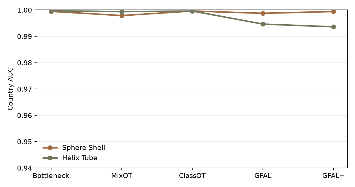
Figure 4 · Final learned manifold codes
The final country code follows the assigned inner/outer manifold structure in both geometries.
Loading final manifold codes…
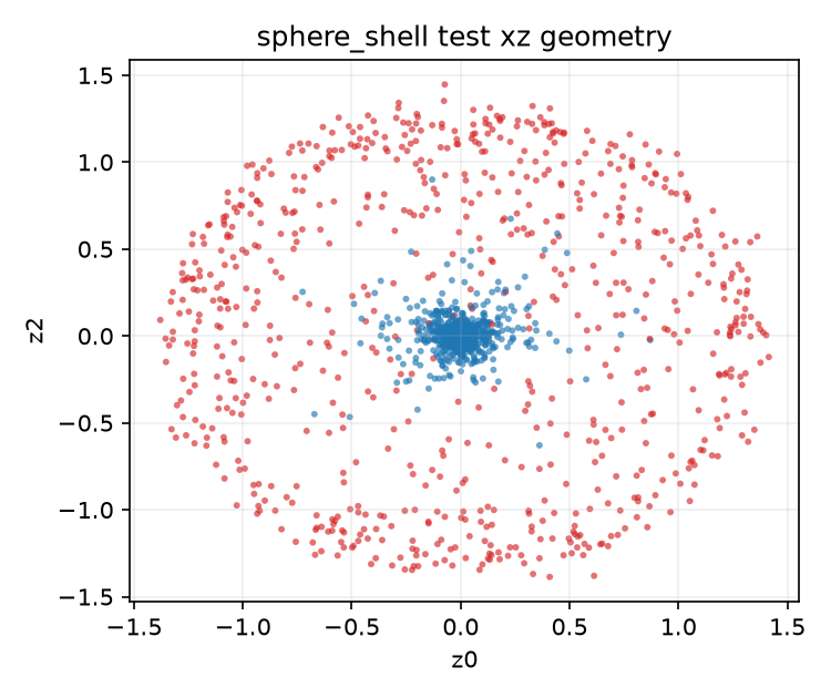
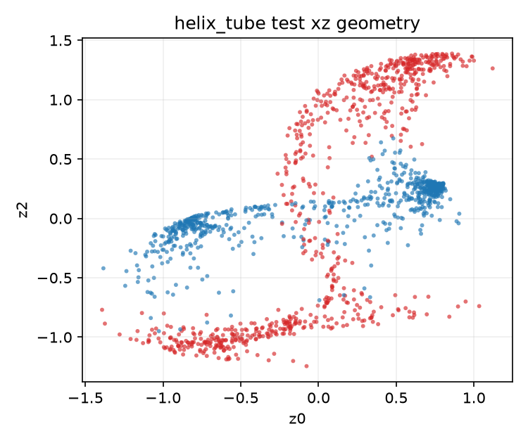
GFAL+ preserves task performance, strong geometry probes, and causal geometry for both manifolds. Its complement result is asymmetric: complement AUC falls from $0.6030$ to $0.5661$ for the helix, but rises from $0.5764$ to $0.6086$ for the sphere.
Thus GFAL+ reduces a complement backup route for the helix but does not establish perfect information isolation for either geometry. The intended geometry remains a strong, causally active pathway, while the complement is not eliminated as an alternative source of country information.
3. Causal-Use Validation
If I edit only the geometry channels after training, does the trained classifier actually follow that edit?
The earlier probes show that the geometry channels contain country information. They do not show that the trained classifier uses them. I therefore freeze the model, select a balanced held-out subset, and edit only the hidden2 geometry channels.
I use four interventions, each asking a different causal question:
- Ablation: set $z_i$ to zero and ask whether country prediction worsens;
- Replacement: insert positive or negative anchors and ask whether the country logit follows;
- Swap: exchange learned geometry codes between labels and ask whether predictions move in the expected directions;
- Path: move smoothly from positive to negative geometry and ask whether the country logit changes smoothly.
For replacement and swap, I also measure specificity: whether country moves much more than the other seven output logits.
3.1 Ablation
I replace $z_i$ with zero, then compute target AUC. The ablation AUC drop is:
\[\operatorname{AUC}_{\text{base}}-\operatorname{AUC}_{\text{ablated}}\]If I remove the geometry signal, does country prediction get worse?
3.2 Replacement
Replacement uses the causal target delta introduced in Section 2.5.1. I replace the learned geometry with a positive or negative anchor while preserving the original complement:
\[h_i^2\to\tilde h_i^2=[\alpha_i^1+b_{\mathcal{G}},r_i], \quad\text{or}\quad h_i^2\to\tilde h_i^2=[\alpha_i^0+b_{\mathcal{G}},r_i]\]Here $\tilde h_i^2$ is the intervened hidden2 state. Because $r_i$ is copied from the original example, the replacement geometry is the only intended cause of output movement. The causal target delta is
\[\Delta_{\text{target}}=\frac{1}{N}\sum_i\left[C_{f^\star}([\alpha_i^1+b_{\mathcal{G}},r_i])-C_{f^\star}([\alpha_i^0+b_{\mathcal{G}},r_i])\right]\]where $C_{f^\star}(h)$ is the country logit by the model tail from hidden2.
3.3 Swap
For positive-negative pairs $(p_j,n_j)$ from the held-out set, I exchange only their learned geometry channels. Let $P$ and $N$ be the selected positive and negative indices. The original hidden states are:
\[h_{p_j}^2=[z_{p_j}+b_{\mathcal G},r_{p_j}],\quad h_{n_j}^2=[z_{n_j}+b_{\mathcal G},r_{n_j}]\]Now swap only the geometry channels:
\[\tilde h_{p_j}^2=[z_{n_j}+b_{\mathcal G},r_{p_j}],\quad\tilde h_{n_j}^2=[z_{p_j}+b_{\mathcal G},r_{n_j}]\]The swap target shift is:
\[\Delta_{\text{swap}}=\frac{1}{2m}\sum_{j=1}^{m}\left[C_{f^\star}(h_{p_j}^2)-C_{f^\star}(\tilde h_{p_j}^2)+C_{f^\star}(\tilde h_{n_j}^2)-C_{f^\star}(h_{n_j}^2)\right]\]where $m$ is the number of positive-negative pairs. The score is high when negative geometry lowers positive examples and positive geometry raises negative examples.
3.4 Path
I choose a deterministic path through the target geometry from the positive radius to the negative radius:
\[z^{(1)},z^{(2)},\ldots,z^{(K)}\]The intuition is that, rather than jumping directly from a positive geometry point to a negative geometry point, I draw a small line or curve of intermediate geometry points between them and check whether the model’s country logit changes smoothly along the way. In both geometries, the label is mainly carried by radius: positives lie at smaller radii and negatives at larger radii. I fix the start point and change only the radius step by step.
For the sphere shell, I pick one direction, such as the positive x-axis, then use radii from the positive to the negative radius $r_1 < \text{…} < r_K$. The model therefore sees an inner shell point, then gradually larger shell points, then an outer shell point.
For the helix tube, I fix one position along the helix core and one tube angle, then increase only the tube radius. I use the same fixed direction or helix position for every evaluation, sweeping radius from the positive-class value to the negative-class value.
I then hold the complement channels at the mean complement $\bar r$ and form:
\[h^{(k)}=[z^{(k)}+b_{\mathcal G},\bar r]\]Let $\ell_k=C_{f^\star}(h^{(k)})$ be the country logit at step $k$. Since the path moves from positive geometry to negative geometry, the expected behavior is that country logit decreases. The path target delta is
\[\Delta_{\text{path}}=\ell_1-\ell_K\]The path monotonic fraction is:
\[M_{\text{path}}=\frac{1}{K-1}\sum_{k=1}^{K-1}\mathbf{1}\left[\ell_k-\ell_{k+1}>0\right]\]$M_{\text{path}}=1$ means every adjacent step moved in the expected direction.
3.5 Specificity
Specificity accompanies the replacement and swap checks. It compares country movement with average off-target movement:
\[\operatorname{specificity}=\frac{|\Delta_{\text{target}}|}{\frac{1}{7N}\sum_i\sum_{f\ne f^\star}\left|C_f([\alpha_i^1+b_{\mathcal{G}},r_i])-C_f([\alpha_i^0+b_{\mathcal{G}},r_i])\right|}\]The denominator is the average movement of the other 7 logits. A high specificity ratio means the geometry edit mainly affects country, not every feature at once.
3.6 Results
Table 6. Causal-use validation on the trained model from the previous stage.
| Geometry | Ablation AUC drop |
Ablation target AUC |
Causal delta |
Swap target shift |
Swap specificity |
Path target delta |
Path monotonic fraction |
Specificity ratio |
|---|---|---|---|---|---|---|---|---|
| Sphere shell | 0.4675 | 0.5317 | 3.5004 | 4.4433 | 92.0223 | 3.4963 | 1.0000 | 73.4252 |
| Helix tube | 0.4279 | 0.5654 | 2.6884 | 7.1863 | 128.0430 | 5.1727 | 1.0000 | 47.3151 |
Figure 5 · Causal-use validation
Each check changes only the three reserved geometry channels, then asks whether the frozen classifier responds in the predicted direction.
Loading causal-use evidence…
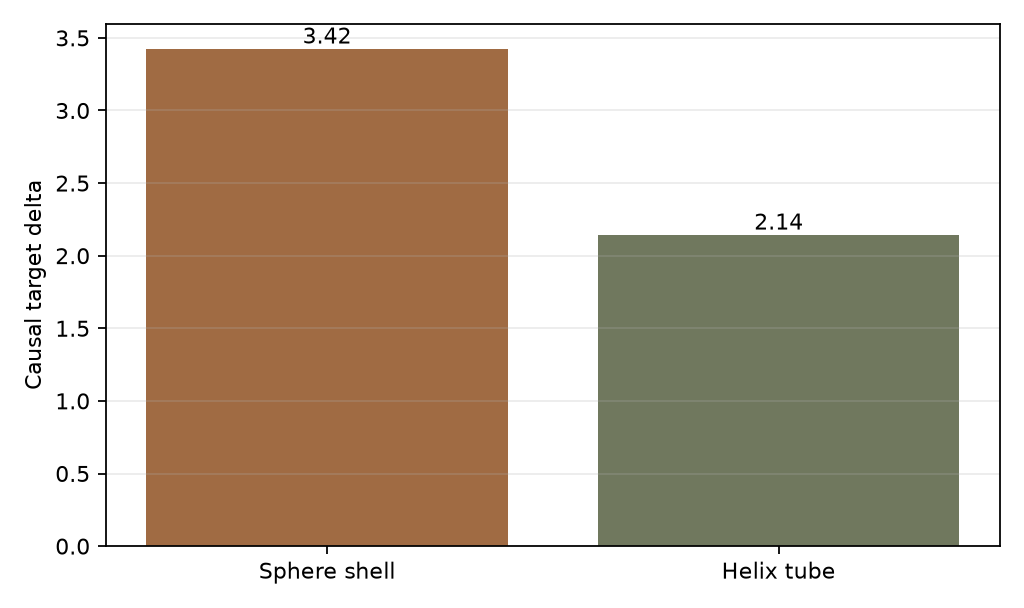
Both geometries pass every check in Table 6. Ablation nearly removes country prediction: the AUC drops by $0.4675$ for the sphere and $0.4279$ for the helix, leaving both close to chance. Replacement moves the country logit in the expected direction, with high specificity ratios of $73.4252$ and $47.3151$ respectively. Each path has a monotonic fraction of $1.0000$, so increasing radius moves the country logit in the expected direction at every step.
The swap check is the strongest learned-code test because it exchanges the model’s own geometry codes rather than synthetic anchors. It produces target shifts of $4.4433$ for the sphere and $7.1863$ for the helix, with specificity ratios of $92.0223$ and $128.0430$. Thus, the learned geometry is not merely visually aligned with country: moving it between examples changes the model’s own prediction path as expected.
The sphere remains geometrically stronger than the helix, with higher coverage entropy and lower radius MAE, but both have strong causal-use evidence. These tests establish a causally active geometry pathway, not perfect information isolation: as Section 2.6 shows, the complement can still retain an alternative source of country information.
References
- Gurnee et al. When Models Manipulate Manifolds: The Geometry of a Counting Task.
- Wurgaft et al. Manifold Steering Reveals the Shared Geometry of Neural Network Representation and Behavior.
- Tolstikhin et al. Wasserstein Auto-Encoders.
- ProofWiki. Variance of Continuous Uniform Distribution.
- Cuturi. Sinkhorn Distances: Lightspeed Computation of Optimal Transportation Distances.
- Geiger et al. Inducing Causal Structure for Interpretable Neural Networks.
- Geiger et al. Causal Abstractions of Neural Networks.
- Ganin et al. Domain-Adversarial Training of Neural Networks.