This is the first of two articles on BlueDot Technical AI Safety Puzzle #1. For the final task, see Can We Teach a Model to Encode a Semantic Feature on a Chosen Manifold in Just Three Channels?.
Takeaway
Country is not linearly accessible at layer $\ell$, but the model’s frozen tail still decodes it almost perfectly. The evidence points to an inside/outside, basin-like representation rather than one global direction.
- Linear probe
- 0.473 AUC
- Frozen tail
- 0.9938 AUC
- Mahalanobis radius
- 0.9941 AUC
About BlueDot’s Puzzle #1
BlueDot’s Technical AI Safety Puzzle #1 provides a trained 5-layer MLP that performs multi-class classification over eight binary features using mean-pooled representations from a sentence transformer. The puzzle indicates nonlinear behavior at the output of the third ReLU, denoted as $\ell$, and asks participants to:
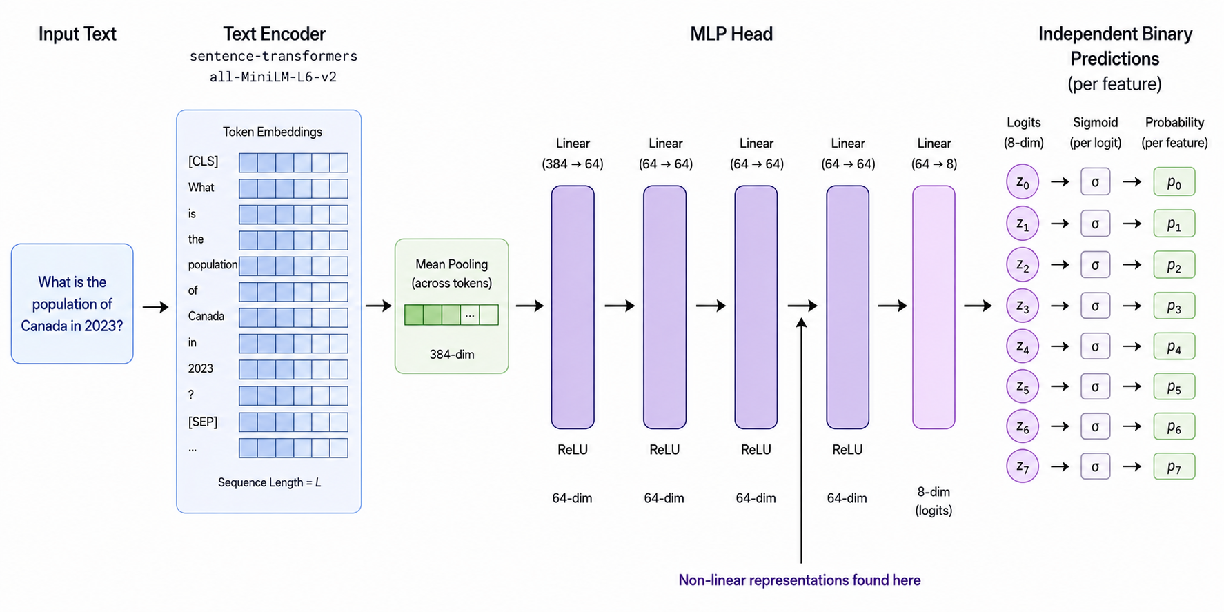
- Find the nonlinear feature, denoted as $f$.
- Explain the geometry used by the model at $\ell$ to represent $f$.
- Train a new model with a more interpretable representation.
This article addresses the first two tasks: identifying the nonlinear feature and explaining its basin-like representation. The companion article trains a new model with a chosen manifold representation.
1. Finding the Nonlinear Feature
1.1 Why Linear Probe (LP)?
The puzzle suggests that one feature $f$ is nonlinear at layer $\ell$. I begin with the simplest competing hypothesis: a single linear direction in the layer-$\ell$ activations is sufficient to recover each feature. I test that hypothesis with a linear probe (LP) [1], [2].
Given activations and their corresponding binary feature labels, an LP asks whether a linear separator can predict a feature from the activations extracted at layer $\ell$.
If a feature is accurately predicted by an LP, its representation at $\ell$ is likely linearly separable. If one feature consistently resists linear classification while the others are easily separated, that is strong evidence for a nonlinear representation.
1.2 Experiment Settings and Metrics
For each feature, I train an independent logistic-regression LP with an L2 penalty on the activations at layer $\ell$ to predict the corresponding binary label.
Using the provided test set, I evaluate recovery and separation:
- Recovery — LP AUC and LP accuracy: LP AUC measures how well the probe ranks positive examples above negative examples across all thresholds; LP accuracy is the fraction of correct predictions.
- Separation — margin gap and overlap: margin gap is the distance between the average positive- and negative-class decision scores, while overlap is the fraction of examples on the wrong side of the decision boundary. A larger gap and lower overlap indicate cleaner linear separation.
1.3 Results
Table 1. LP AUC, LP accuracy, margin gap, and overlap of the eight trained probes for each feature.
| Feature | LP AUC ↑ | LP accuracy ↑ | Margin Gap ↑ | Overlap ↓ |
|---|---|---|---|---|
| sentiment | 0.995 | 0.982 | 11.385 | 0.018 |
| food | 0.996 | 0.985 | 19.136 | 0.014 |
| color | 0.997 | 0.971 | 10.775 | 0.028 |
| number | 0.997 | 0.975 | 11.298 | 0.024 |
| body part | 0.998 | 0.980 | 10.550 | 0.020 |
| person | 0.999 | 0.998 | 11.434 | 0.002 |
| country | 0.473 | 0.489 | 0.00015 | 0.511 |
Table 1 shows that seven features are recovered almost perfectly by their LPs: each has LP AUC of at least 0.995 and a large decision margin.
The exception is country. Its LP AUC (0.473) and LP accuracy (0.489) are near chance, its margin gap is nearly zero, and 0.511 of test examples fall on the wrong side of the decision boundary. This is a sharp failure of linear separation rather than a small degradation relative to the other features.
This makes country the leading nonlinear candidate at layer $\ell$, but LP failure alone does not show whether the information is absent or merely nonlinearly encoded. I therefore run two sanity checks.
1.4 Sanity Check 1: Tail Sanity Check
An LP failure cannot distinguish between two possibilities:
- The feature is nonlinear.
- The feature is not present.
The frozen-tail check asks whether the model’s original tail can still predict country from the layer $\ell$ activations. High tail AUC and accuracy would show that the information is present at $\ell$ and decoded nonlinearly downstream.
It also catches implementation errors such as extracting the wrong layer, misordering features, shuffling activations against labels, or batching mismatches.
The frozen tail reaches 0.9938 AUC and 0.9640 accuracy for country on 1,500 test examples. The country signal is therefore still usable from the extracted activations, even though a separately trained LP cannot recover it.
1.5 Sanity Check 2: Causal Steering
I test the same hypothesis from a complementary angle. A linearly represented feature should have a meaningful global direction: moving activations along that direction should systematically change the corresponding feature logit [3]. For each steering feature $k$, I define a candidate direction:
\[d_k = \mu_{k,1} - \mu_{k,0},\]where $\mu_{k,1}$ is the mean layer $\ell$ activation for positive examples of feature $k$, and $\mu_{k,0}$ is the mean for negative examples.
I then intervene on the layer $\ell$ activations as:
\[h' = h + \alpha \hat d_k, \quad \hat d_k = \frac{d_k}{\lVert d_k \rVert},\]where $\alpha \in [-5,5]$ is the steering strength, before passing the activations through the remaining model tail.
For a linear feature, increasing $\alpha$ should produce a consistent change in the feature logit. A weaker or less consistent response suggests that the feature is not controlled by one global direction, but by a more structured or multi-region representation.
Metrics. Let $C_{f}(\cdot)$ be the model’s logit for feature $f$,
\[\bar C_f^{(k)}(\alpha)=\frac{1}{N_{\text{test}}}\sum_{i}C_f(h_i+\alpha \hat d_k)\]Here $k$ is the feature whose direction is steered and $f$ is the measured output logit. Across a fixed $\alpha$ grid, I measure:
- Monotonicity: whether the target score moves in the intended direction as steering strength increases; specifically, the fraction of adjacent steps where
- Target logit delta: the signed target-logit change between $\alpha=-5$ and $\alpha=5$:
- Max off-target delta: the largest unintended absolute change among all other features:
- Specificity ratio: the ratio of target-logit delta to maximum off-target delta, summarizing whether the target movement is large relative to its largest side effect.
Table 2. Causal steering behavior among the features.
| Feature | Monotonicity ↑ | Target logit delta ↑ | Max off-target delta ↓ | Specificity ratio ↑ |
|---|---|---|---|---|
| number | 1.00 | 132.9 | 19.2 | 6.9 |
| question | 1.00 | 217.2 | 27.8 | 7.8 |
| color | 1.00 | 179.3 | 19.9 | 8.9 |
| food | 1.00 | 269.5 | 14.4 | 18.6 |
| sentiment | 1.00 | 344.3 | 19.1 | 17.9 |
| country | 0.51 | 14.9 | 197.2 | 0.07 |
| person | 1.00 | 131.5 | 8.3 | 15.8 |
| body part | 1.00 | 169.6 | 25.8 | 6.6 |
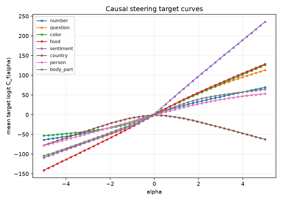
Table 2 and Figure 1 show the expected simple-direction behavior for the non-country features: every curve is perfectly monotonic, and each target movement is much larger than its largest off-target effect. For example, food has a target delta of 269.5, a maximum off-target delta of 14.4, and a specificity ratio of 18.6.
Country again breaks the pattern. Its target-logit monotonicity is 0.51, its endpoint target-logit delta is only 14.9, and its largest off-target movement is 197.2. Thus, the normalized country direction changes another logit far more than it changes country itself, yielding a specificity ratio of 0.07 while every other feature exceeds 6.5.
Figure 1 · Causal steering curves
Country reverses direction while the linear controls move smoothly with $\alpha$.
Loading causal-steering data…
1.6 Question 1 Conclusion
The feature most likely to be represented nonlinearly is country.
At layer $\ell$, seven features behave as linearly accessible directions: LPs recover them, and steering along their class-mean directions causally moves the matching downstream logits. Country breaks both patterns. Its LP is near chance, its class-mean direction has little useful effect on its own logit, and steering mainly changes other outputs. Yet the frozen downstream tail still predicts country accurately, so the information is present but not encoded as one global linear direction.
2. Explaining the Country Basin
2.1 Basin Hypothesis
Country is not represented as a linear region. It is closer to an inside/outside region, or a basin-like region, in the layer $\ell$ activation space.
Question 1 leaves a puzzle: a linear probe cannot recover country from layer $\ell$, but the original model tail can. I therefore test whether the ReLU tail decodes country with different local directions in different regions of activation space.
The tail is piecewise linear: near one hidden state $h$, its ReLU on/off pattern is fixed and the feature logit has one local direction; near another state, that pattern can change and so can the direction. Several local halfspaces can therefore form a curved boundary [4]. The analyses below test this decoder hypothesis, then ask whether the activations themselves form the predicted inside/outside region.
For a feature $f$ logit, the remaining tail is roughly:
\[z_f(h)=w_f^\top \operatorname{ReLU}(Ah+b)+c_f\]Then the local gradient is:
\[g_f(h)=\nabla_h z_f(h)=w_f^\top \operatorname{diag}(\mathbf{1}_{Ah+b>0})A\]This is the direction that most rapidly increases a feature score around $h$, through the currently active pathways $\operatorname{diag}(\mathbf{1}_{Ah+b>0})$. It is similar in spirit to class-score gradients used to inspect directions that support a class [5]. A linear feature should reuse nearly one direction; a nonlinear feature should rotate, split, or spread across examples.
2.2 Measurements
I use extracted hidden-2 post-ReLU test activations throughout. The analysis proceeds in three steps:
- Local gradient cosine asks whether the decoder reuses one direction across examples.
- Gradient PCA shows how those local directions vary across features.
- Representation geometry asks where the corresponding layer $\ell$ activations lie in a decoder-relevant 3D view.
2.3 Local Gradient Consistency
For each feature, I normalize every local gradient:
\[\hat g_f(h_i)=\frac{g_f(h_i)}{\lVert g_f(h_i) \rVert+\epsilon}\]Then I compute the mean pairwise cosine between local gradients:
\[\kappa_f=\frac{1}{N(N-1)}\sum_{i\ne j}\hat g_f(h_i)^\top \hat g_f(h_j)\]Values close to 1 indicate one reusable local direction; much lower values indicate that the decoder changes direction across ReLU regions.
Table 3. Local gradient consistency of all eight features.
| Feature | Mean normalized local gradient cosine ↑ |
|---|---|
| color | 0.9862 |
| body part | 0.9862 |
| person | 0.9840 |
| question | 0.9830 |
| number | 0.9823 |
| food | 0.9600 |
| sentiment | 0.8898 |
| country | 0.5442 |
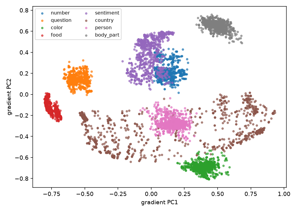
Most features are stable, with local-gradient cosines between 0.9600 and 0.9862; even sentiment reaches 0.8898. Country is the exception at 0.5442, indicating that the model uses different country directions in different local regions.
2.4 Gradient PCA
To compare local directions directly, I stack the normalized gradients for all features and fit one shared PCA:
\[G_{\mathrm{all}}=\{\hat g_f(h_i): f\in \text{features}, i\in \text{test examples}\}\] \[Z=\operatorname{PCA}_2(G_{\mathrm{all}})\]Each feature is then plotted in this same 2D space. Linear features should form tight clusters, whereas country should spread out or split because it uses several directions.
For each feature cloud, I then compute its centroid and the radius of each point:
\[\bar z_f=\frac{1}{N_f}\sum_{i:y_i=f} z_{i}, \quad r_i=\lVert z_i-\bar z_f \rVert_2\]I summarize each cloud by its mean and 95% radius.
Table 4. Mean radius and 95% radius of each feature after 2D PCA projection.
| Feature | Mean radius ↓ | 95% radius ↓ |
|---|---|---|
| number | 0.070 | 0.169 |
| question | 0.060 | 0.116 |
| color | 0.054 | 0.125 |
| food | 0.065 | 0.124 |
| sentiment | 0.153 | 0.284 |
| country | 0.530 | 0.696 |
| person | 0.067 | 0.150 |
| body part | 0.061 | 0.115 |
The other features form tight clouds: their local arrows point to roughly the same place. Country instead forms a broad curved band. This shared PCA uses 12,000 normalized gradients (8 features × 1,500 test samples).
Figure 2 · Shared gradient-PCA view
A shared projection of 12,000 local gradients, with country brought forward.
Loading gradient-PCA data…
2.5 Looking at the Activations
Gradient PCA describes the decoder; I next examine the representation itself. For each feature $f$, I project activations into a feature-specific 3D subspace fitted from its normalized local gradients, rather than a basis chosen only for raw activation variance. The question is: in the directions selected by the local decoder geometry, what shape do the layer $\ell$ activations take?
For a feature $f$, I take its usable normalized local gradients $G_f={\hat g_f(h_i)}_{i=1}^{N}$. Then I fit a 3D PCA basis on those gradients
\[U_f=\operatorname{PCA}_3(G_f)\]and project the test activations into the corresponding feature-specific basis after removing the mean:
\[q_{i,f}=U_f(h_i-\bar h_f)\]Figure 3 · Decoder-relevant activation projections
Country concentrates around a central region, unlike the linear body-part control.
Loading representation data…
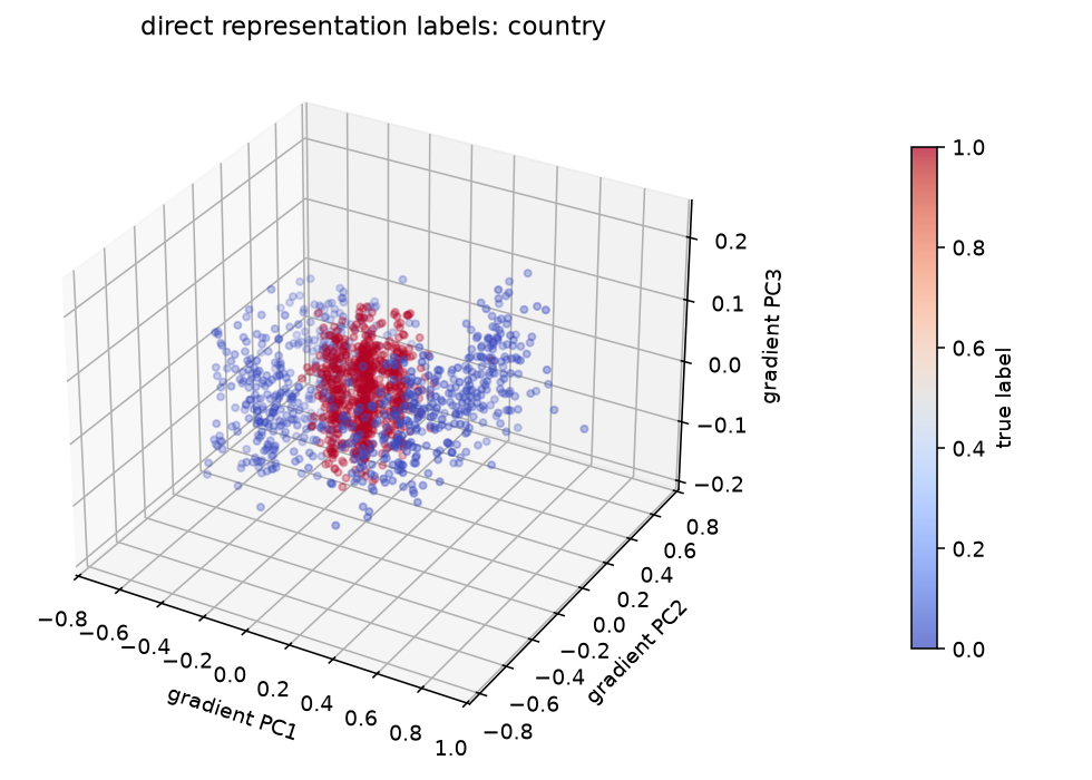
This is the first plot where the representation becomes visible. I expected a messy split into several clusters; instead, country-positive examples concentrate near a central region while many negative examples sit around the outside.
→ This suggests that country is represented inside a basin-like region.
One caveat is that these visualizations do not show the full manifold. The representation is still 64-dimensional, and this is only a decoder-relevant 3D view.
2.6 Radius and Mahalanobis Sanity Check
If country is an inside / basin-like region, can distance from the center recover it?
I fit the geometry on training data and score held-out test data. The 3D gradient basis is fitted from training hidden-2-post-ReLU activations and local gradients, then applied to test activations.
\[U_c=\operatorname{PCA}_3(\{\hat g_c(h_i)\}_{i\in\mathrm{train}}), \quad z_i=U_c^\top(h_i-\bar h_{\mathrm{train}})\]I turn “inside the basin” into two complementary distance scores:
- Euclidean radius is the circular-basin check, using the projected origin $r_i=\lVert z_i \rVert_2$. If country positives lie near the center, smaller radius should indicate country.
- Mahalanobis radius is the elliptical-basin check. I fit the positive samples’ mean and covariance in the first two projected dimensions.
It measures distance from the positive center while accounting for the positive class’s shape: distance along a naturally wide direction counts less than distance along a tight one.
\[m_i=\sqrt{(z_{i,1:2}-\mu_+)^\top\Sigma_+^{-1}(z_{i,1:2}-\mu_+)}\]The score is:
\[s^{\mathrm{maha}}_i=-m_i\]Table 5 compares these basin scores with a linear probe, a quadratic probe, and the frozen tail from Section 1.4. The quadratic probe uses linear, squared, and pairwise-product terms:
For the quadratic probe I used:
\[\phi(z)=[z_1,z_2,z_3,z_1^2,z_2^2,z_3^2,z_1z_2,z_1z_3,z_2z_3]\]Table 5. Country AUC of five different probes.
| Method | Country AUC ↑ |
|---|---|
| Linear probe | 0.4959 |
| Euclidean radius | 0.9930 |
| Mahalanobis radius | 0.9941 |
| Quadratic probe | 0.9936 |
| Frozen tail | 0.9938 |
Figure 4 · Country radial basin and food control
Compare the country basin against food in the same diagnostic.
Loading radial-basin data…
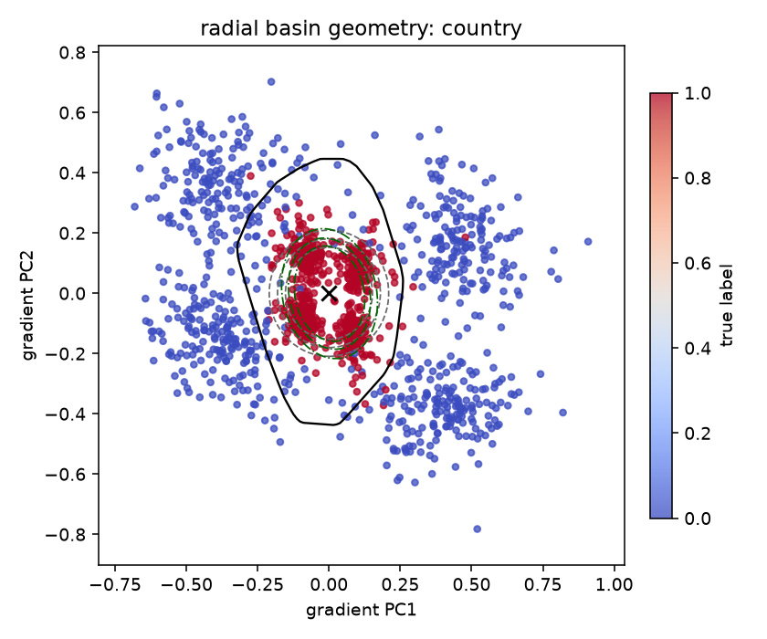
Table 5 and Figure 4 agree: country-positive examples concentrate near the center in the country tail-gradient projection. Radius and Mahalanobis scores recover country almost as well as the frozen tail, while the linear probe remains at chance. The same diagnostic does not separate food, suggesting that the radius effect is country-specific rather than a generic projection artifact.
2.7 Score Landscape
As a complementary diagnostic, I ask: what does the frozen tail’s country score look like on a simple activation plane? If country were linear, the tail should resemble one tilted plane on this slice. This view cannot prove the full 64D representation, but it can show why a single linear boundary is implausible.
I first chose a shared activation plane:
\[h(x,y)=h_0+xu_1+yu_2\]where $u_1$ and $u_2$ are the first two activation-PCA directions. I then evaluate the frozen tail’s country logit:
\[C_c(x,y)=C_c(h(x,y))\]The zero contour is
\[\Gamma_c=\{(x,y): C_c(x,y)=0\}\]Figure 5 · Score landscapes
Country’s surface folds; the linear controls remain close to planes.
Loading score-landscape data…
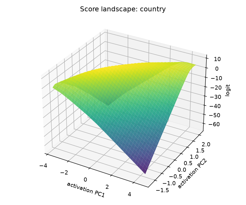
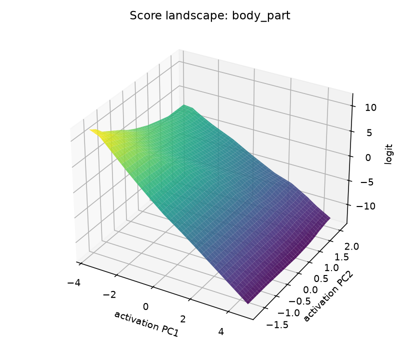
The country landscape is curved, whereas body part—and the other six labels—forms a tilted plane. Country also has the most fragmented zero contour, with 274 segments. Its positive and negative class centroids in this shared plane are almost identical (distance 0.058). Together, these observations show that the tail creates a nonlinear high-score region around country-positive activations.
References
- Giulianelli et al. Under the Hood: Using Diagnostic Classifiers to Investigate and Improve how Language Models Track Agreement Information.
- Pimentel et al. Information-Theoretic Probing for Linguistic Structure.
- Kim et al. Interpretability Beyond Feature Attribution: Quantitative Testing with Concept Activation Vectors (TCAV).
- Montufar et al. On the Number of Linear Regions of Deep Neural Networks.
- Simonyan et al. Deep Inside Convolutional Networks: Visualising Image Classification Models and Saliency Maps.